先用最简单的三层全连接神经网络,然后添加激活层查看实验结果,最后加上批标准化验证是否有效
<强>首先根据已有的模板定义网络结构SimpleNet,命名py为
进口火炬
从火炬。autograd导入变量
进口numpy np
进口matplotlib。pyplot作为plt
从火炬进口nn, optim
从torch.utils。数据导入DataLoader
从torchvision导入数据,转换
#定义三层全连接神经网络
类simpleNet (nn.Module):
def __init__(自我、in_dim n_hidden_1、n_hidden_2 out_dim): #输入维度,第一层的神经元个数,第二层的神经元个数,以及第三层的神经元个数
超级(simpleNet自我). __init__ ()
self.layer1=nn.Linear (in_dim n_hidden_1)
self.layer2=nn.Linear (n_hidden_1 n_hidden_2)
self.layer3=nn.Linear (n_hidden_2 out_dim)
def向前(自我,x):
x=self.layer1 (x)
x=self.layer2 (x)
x=self.layer3 (x)
返回x
#添加激活函数
类Activation_Net (nn.Module):
def __init__(自我、in_dim n_hidden_1、n_hidden_2 out_dim):
超级(NeutalNetwork自我). __init__ ()
self.layer1=nn.Sequential(#顺序组合结构
nn.Linear (in_dim n_hidden_1) nn.ReLU(真正的))
self.layer2=nn.Sequential (
nn.Linear (n_hidden_1 n_hidden_2) nn.ReLU(真正的))
self.layer3=nn.Sequential (
nn.Linear (n_hidden_2 out_dim))
def向前(自我,x):
x=self.layer1 (x)
x=self.layer2 (x)
x=self.layer3 (x)
返回x
#添加批标准化处理模块,皮标准化放在全连接的后面,非线性的前面
类Batch_Net (nn.Module):
def _init__(自我、in_dim n_hidden_1、n_hidden_2 out_dim):
超级(Batch_net自我). __init__ ()
self.layer1=nn.Sequential (nn.Linear (in_dim n_hidden_1) nn.BatchNormld (n_hidden_1) nn.ReLU(真正的))
self.layer2=nn.Sequential (nn.Linear (n_hidden_1 n_hidden_2) nn.BatchNormld (n_hidden_2) nn.ReLU(真正的))
self.layer3=nn.Sequential (nn.Linear (n_hidden_2 out_dim))
def丰华(自我,x):
x=self.layer1 (x)
x=self.layer2 (x)
x=self.layer3 (x)
返回x
之前
<>强训练网络,
进口火炬
从火炬。autograd导入变量
进口numpy np
进口matplotlib。pyplot作为plt
% matplotlib内联
从火炬进口nn, optim
从torch.utils。数据导入DataLoader
从torchvision导入数据,转换
#定义一些超参数
净进口
batch_size=64
learning_rate=1依照
num_epoches=20
#预处理
data_tf=transforms.Compose (
[transforms.ToTensor (), transforms.Normalize([0.5],[0.5])]) #将图像转化成张量,然后继续标准化,就是减均值,除以方差
#读取数据集
train_dataset=datasets.MNIST (root=啊?数据”,火车=True,变换=data_tf下载=True)
test_dataset=datasets.MNIST (root=啊?数据”,火车=False,变换=data_tf)
#使用内置的函数导入数据集
train_loader=DataLoader (train_dataset batch_size=batch_size洗牌=True)
test_loader=DataLoader (test_dataset batch_size=batch_size洗牌=False)
#导入网络,定义损失函数和优化方法
模型=net.simpleNet (28 * 28300100, 10)
如果torch.cuda.is_available(): #是否使用cuda加速
模型=model.cuda ()
标准=nn.CrossEntropyLoss ()
优化器=optim.SGD (model.parameters (), lr=learning_rate)
净进口
n_epochs=5
时代的范围(n_epochs):
running_loss=0.0
running_correct=0
print(“时代{}/{}”.format(时代,n_epochs))
打印(“-”* 10)
在train_loader数据:
img标签=数据
img=img.view (img.size (0) 1)
如果torch.cuda.is_available ():
img=img.cuda ()
标签=label.cuda ()
其他:
img=变量(img)
标签=变量(标签)=模型(img) #得到前向传播的结果
损失=标准(标签),#得到损失函数
print_loss=loss.data.item ()
optimizer.zero_grad() #归0梯度
loss.backward() #反向传播
optimizer.step() #优化
running_loss +=loss.item ()
时代+=1
如果时代% 50==0:
打印(“时代:{},失:{:.4f} .format(时代,loss.data.item ()))
之前
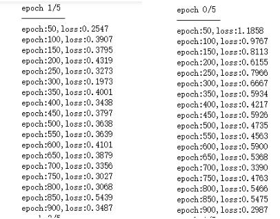
训练的结果截图如下:
<强>测试网络
#测试网络
model.eval() #将模型变成测试模式
eval_loss=0
eval_acc=0
在test_loader数据:
img标签=数据
img=img.view (img.size(0) 1) #测试集不需要反向传播,所以可以在前项传播的时候释放内存,节约内存空间
如果torch.cuda.is_available ():
img=变量(img,挥发性=True) .cuda ()
标签=变量(标签,挥发性=True) .cuda ()
其他:
img=变量(img,挥发性=True)
标签=变量(标签,挥发性=True)=模型(img)
损失=标准(标签),
eval_loss +=loss.item () * label.size (0)
_,pred=torch.max (, 1)
num_correct=(pred==标签).sum ()
eval_acc +=num_correct.item ()
打印(“测试损失:{:.6f}, ac: {: .6f} .format (eval_loss/(len (test_dataset)), eval_acc/(len (test_dataset))))