scikit-learn是python的第三方机器学习库,里面集成了大量机器学习的常用方法,例如:贝叶斯,支持向量机,资讯等。
scikit-learn的官网:http://scikit-learn.org/stable/index.html点击打开链接
SVR是支持向量回归(支持向量回归)的英文缩写,是支持向量机(SVM)的重要的应用分支。
scikit-learn中提供了基于libsvm的SVR解决方案。
PS: libsvm是台湾大学林智仁教授等开发设计的一个简单,易于使用和快速有效的SVM模式识别与回归的软件包。
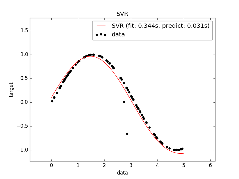
我们自己随机产生一些值,然后使用罪函数进行映射,使用SVR对数据进行拟合
然后我们对结果进行可视化处理
 ##############################################################################
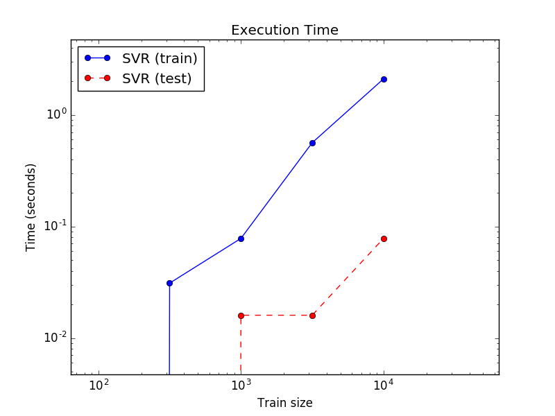
#对训练和测试的过程耗时进行可视化
X=5 * rng。兰特(1000000 1)
y=np.sin (X) .ravel ()
y (:: 50) +=2 * (0.5 - rng.rand (int (X.shape [0]/50)))
大?np。logspace (1、4、7)
的名字,估计在{
“SVR”: SVR(内核=rbf, C=1 e1,γ=10)}. items ():
train_time=[]
test_time=[]
train_test_size的大小:
t0=time.time ()
estimator.fit (X [: int (train_test_size)], [: int (train_test_size)])
train_time.append (time.time () - t0)
t0=time.time ()
estimator.predict (X_plot [1000]):
test_time.append (time.time () - t0)
plt。情节(大小、train_time“啊——”,颜色=癰”如果name==癝VR”其他“g”,
label=" % s(火车)”%的名字)
plt。情节(大小、test_time“啊——”,颜色=" r "如果name==癝VR”其他“g”,
标签=" % s(测试)"%的名字)
plt.xscale(“日志”)
plt.yscale(“日志”)
plt。包含(“列车规模”)
plt。ylabel(“时间(秒)”)
plt。标题(“执行时间”)
plt.legend (loc=白詈谩?
##############################################################################
#对训练和测试的过程耗时进行可视化
X=5 * rng。兰特(1000000 1)
y=np.sin (X) .ravel ()
y (:: 50) +=2 * (0.5 - rng.rand (int (X.shape [0]/50)))
大?np。logspace (1、4、7)
的名字,估计在{
“SVR”: SVR(内核=rbf, C=1 e1,γ=10)}. items ():
train_time=[]
test_time=[]
train_test_size的大小:
t0=time.time ()
estimator.fit (X [: int (train_test_size)], [: int (train_test_size)])
train_time.append (time.time () - t0)
t0=time.time ()
estimator.predict (X_plot [1000]):
test_time.append (time.time () - t0)
plt。情节(大小、train_time“啊——”,颜色=癰”如果name==癝VR”其他“g”,
label=" % s(火车)”%的名字)
plt。情节(大小、test_time“啊——”,颜色=" r "如果name==癝VR”其他“g”,
标签=" % s(测试)"%的名字)
plt.xscale(“日志”)
plt.yscale(“日志”)
plt。包含(“列车规模”)
plt。ylabel(“时间(秒)”)
plt。标题(“执行时间”)
plt.legend (loc=白詈谩?
 ################################################################################
#对学习过程进行可视化
plt.figure ()
svr=svr(内核=rbf, C=1 e1,γ=0.1)
train_sizes、train_scores_svr test_scores_svr=\
learning_curve (svr, X [100], [100], train_sizes=np.linspace (0.1 1 10),
得分=" neg_mean_squared_error ",简历=10)
plt。情节(train_sizes -test_scores_svr.mean(1),“啊——”,颜色=" r ",
标签=癝VR”)
plt。包含(“列车规模”)
plt。ylabel(均方误差)
plt。标题(“学习曲线”)
plt.legend (loc=白詈谩?
plt.show ()
################################################################################
#对学习过程进行可视化
plt.figure ()
svr=svr(内核=rbf, C=1 e1,γ=0.1)
train_sizes、train_scores_svr test_scores_svr=\
learning_curve (svr, X [100], [100], train_sizes=np.linspace (0.1 1 10),
得分=" neg_mean_squared_error ",简历=10)
plt。情节(train_sizes -test_scores_svr.mean(1),“啊——”,颜色=" r ",
标签=癝VR”)
plt。包含(“列车规模”)
plt。ylabel(均方误差)
plt。标题(“学习曲线”)
plt.legend (loc=白詈谩?
plt.show ()